Back Propogation

Gradient Descent

Our objective with the gradient descent algorithm is to reach a local minimum in our cost function by tweaking the paramters. While there are several additional improvements and variations of gradient descent like gradient boosting being implemented, the basic algorithm works well in most cases.

---

Intuition

The cost function is a function of the weights and biases of our neural network that measures performace. In the following example, the ellipses are contour lines of an arbitrary cost function. If you are not familiar with what contour lines are, the number next to each line represents the value of the function at every point on that line. So you can think of this graph as getting higher and higher as you go out from the center like a bowl.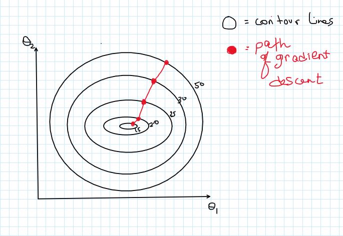 You can see here that we want to tweak \(\theta_1\) and \(\theta_2\) so that we reach a local minimum. If we take the gradient at a point in the graph (which is the slope of the red line), it will point us in the direction of steepest ascent at that point. Therefore, in order to reduce our error, we travel in the direction of the negative gradient, aka steepest descent. So say we start off with some random weights \(\theta_1\) and \(\theta_2\). Each iteration of gradient descent will be as follows:
$$\theta := \theta - \frac{dJ}{d\theta}$$ So every iteration or "epoch", we decrement \(\theta\) by the value of the gradient at that point with respect to \(\theta\) (\(:=\) is the assignment operator).

In Practice

Learning Rate

Usually, when we are performing gradient descent, directly subtracting the gradient is not a good idea because it can be too large or too small(more often the former). Therefore, a "learning rate" is used to scale the gradient and to obtain a better control of the learning process. We use a hyper parameter, \(\alpha \), for this learning rate.
With this in practice, the gradient descent algorithm would look like this:
$$ \theta := \theta - \alpha(\frac{dJ}{d\theta})$$ where \(\alpha \) is a hyperparameter that we pick.

Cost Function

Now that we have a basic grasp of gradient descent, the next task is to pick the right cost function. In our forward pass example, we designed a neural net to predict a continous outcome. We can use the same cost function that the linear regression algorithm uses: Mean Squared Error or MSE. Simply put, we want our neural net to make an approximation of the labels so we can use MSE here. If our task was categorization, the process is slightly more complex.
Mean Squared Error: $$\frac{1}{M} \sum_{i=0}^M(y^{(i)} - a^{(L)}_i)^2$$
Let's break this down: 'M' is the number of samples, \(a^{(L)}_i\) is the output of the neural network for the \(i\)-th sample, \(y^{(i)}\) is the \(i\)-th label. So we are squaring the difference between the prediction and values and taking the average over all samples. Why do we square it? Because if it wasnt, we would see errors cancelling out. So squaring it makes sure error is always positive for every sample.

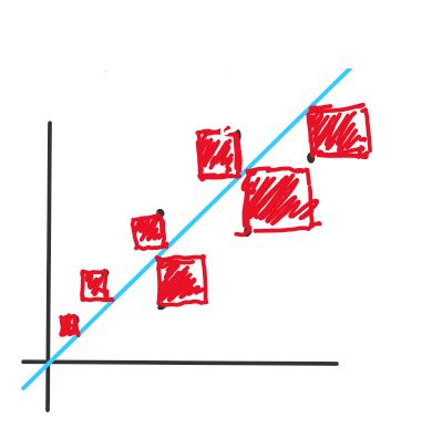
2D visual representation:

Derivative of the Cost Function

The end goal of this is to tweak our parameters so that we can find the perfect amount that we need to "turn the knob" on each parameter. So in order to find \(\frac{dJ}{d\theta}\), we have to apply the chain rule as follows:
$$ \frac{dJ}{dW} = \frac{dJ}{da^{(L)}} * \frac{da^{(L)}}{dz} * \frac{dz}{d\theta}$$
This derivative calculation is for a single layer perceptron and to figure out the weight parameters.
Let's go back to the neural network we used in the other blog: $$ \displaylines{J(\theta) = \frac{1}{M}\sum_{i=0}^M(A_2 - y)^2 \\ \\
\frac{dJ}{dW_2} = \frac{dJ}{dA_2} * \frac{dA_2}{dZ_2} * \frac{dZ_2}{dW_2}\\
\frac{dJ}{dB_2} = \frac{dJ}{dA_2} * \frac{dA_2}{dZ_2} * \frac{dZ_2}{dB_2}\\
\\ \frac{dJ}{dW_1} = \frac{dJ}{dA_2} * \frac{dA_2}{dZ_2} * \frac{dZ_2}{dA_1} * \frac{dA_1}{dZ_1} * \frac{dZ_1}{dW_1}\\
\frac{dJ}{dB_1} = \frac{dJ}{dA_2} * \frac{dA_2}{dZ_2} * \frac{dZ_2}{dA_1} * \frac{dA_1}{dZ_1} * \frac{dZ_1}{dB_1}} $$
Now, let's compute each derivative. I am going to leave out the summation notation for simplicity purposes.

First set of derivatives

$$ \displaylines{\frac{dJ}{dA_2} = 2(A_2 - y)\\
\frac{dA_2}{dZ_2} = A_2(1 - A_2)\longrightarrow\textrm{simplified} \\ \frac{dZ_2}{dW_2} = A_1 \\
\frac{dZ_2}{dB_2} = 1
} $$

Second set of derivatives

Some derivatives we need are already calculated above.

$$ \displaylines{\frac{dZ_2}{dA_1} = W2 \\
\frac{dA_1}{dZ_1} = A_1(1 - A_1) \\
\frac{dZ_1}{dW_1} = X \\
\frac{dZ_1}{dB_1} = 1 }$$ Now, you can plug in these values to get \(\frac{dJ}{dW_2}\),\(\frac{dJ}{dB_2}\),\(\frac{dJ}{dW_1}\),\(\frac{dJ}{dB_1}\).