Forward Propogation

Wow, Neural Networks

Neural Networks are one of the biggest black boxes, yet they are present in every corner of our lives. In essence, they are functions that are able to learn whacky patterns. But what about it makes it a challenge to understand? Is it the heavy calculus involved? “There are so many derivatives to compute". Okay, but if you know this one thing called the Chain Rule, you have the weapon you need to defeat the mini-boss that is calculus.

Linear Algebra.

If you don’t know how to do matrix multiplication or dot products, I suggest you head over to MIT Opencourseware and guzzle their content down because that is an excellent way to build enough confidence to start the vector hell that is Neural Networks. Okay. So if you are confident with vectors, dot products, and matrix multiplication, congratulations. You hold the key to level 1: A 2-Layer Perceptron(composed of a hidden layer and output layer).

Here We Go!

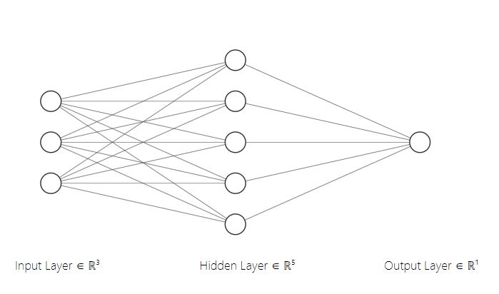
Step 1: Visualize

Let’s say each sample in our training data has 3 features and we have 100 samples. Our hidden layer has 5 neurons and finally our output layer has 1 neuron. One thing to keep in mind is that each neuron produces one output and one output only.

Step 2: Initialize Parameters

import numpy as np
# initialize random data
X = np.random.random((3, 100))
# initialize the first layer
W1 = np.random.random((5, 3))
B1 = np.random.random((5,1))

There are 5 neurons in our hidden layer stacked vertically. The weights that we initialized are also 5 vertically stacked rows of weights. Therefore, each row represents one neuron. Consequently there is 1 bias per neuron/row. You might also be wondering why the weights are 3 x 100 and not 100 x 3. Well, in the visual above, the input features are stacked vertically. So often, you are going to want to transpose your data when you first obtain it raw because each sample is a row in most datasets. Luckily, transposing is super easy in numpy(read the docs).

Next, we will need an activation function for this layer to introduce non-linearity. We will be using the sigmoid activation function. This function will be element-wise, so it will not affect the output's dimensions.

def sigmoid(x):
return 1/(1+np.exp(-x))

Now we will initialize the second/output layer.

W2 = np.random.random((1, 5))
B2 = np.random.random((1,1))

Step 3: Forward Propogation

So in this case, we have one neuron for our output layer. Thus, we use one row of 5 weights for each of the 5 outputs from the previous layer. Now, since we have initialized our weights, we can start forward propagating.

# layer 1
Z1 = W1 @ X + B1
A1 = sigmoid(Z1)
# layer 2
Z2 = W2 @ A1 + B2
A2 = sigmoid(Z2)

That's it!

#Complete Code:
import numpy as np

#Define the activation function
def sigmoid(x):
return 1/(1+np.exp(-x))

# initialize random data
X = np.random.random((3, 100))

# initialize the first layer
W1 = np.random.random((5, 3))
B1 = np.random.random((5, 1))
# initialize the second layer
W2 = np.random.random((1, 5))
B2 = np.random.random((1,1))

# layer 1
Z1 = W1 @ X + B1
A1 = sigmoid(Z1)

# layer 2
Z2 = W2 @ A1 + B2
A2 = sigmoid(Z2)